A Quick Introduction to `ggdag`

Sakeef M. Karim
New York University

CONSORTIUM ON ANALYTICS FOR DATA-DRIVEN DECISION-MAKING

What We’ll Do Today

Install and load the packages you’ll need to generate directed acyclic graphs (DAGs) in .

library(tidyverse)
library(dagitty)
library(ggdag)
library(ggthemes)

Revisit an example from this week’s asynchronous module .
Learn how to use dagitty and ggdag in-tandem.
Use ggdag functions as tools to identify sources of bias.
Customize our DAGs using ggdag functions & ggplot2.

A DAG Example

Show the underlying code

dag_cand3 <- dagitty('dag {
                          Birth_Defects [outcome,pos="0.109,0.631"]
                          Difficulty_Conceiving [pos="0.117,-1.517"]
                          Genetics [pos="0.850,-0.411"]
                          PNC [pos="-0.837,-0.433"]
                          SES [pos="-1.839,-1.468"]
                          Vitamins [exposure,pos="-1.844,0.645"]
                          Difficulty_Conceiving -> PNC
                          Genetics -> Birth_Defects
                          Genetics -> Difficulty_Conceiving
                          PNC -> Birth_Defects
                          PNC -> Vitamins
                          SES -> PNC
                          SES -> Vitamins
                          Vitamins -> Birth_Defects
                          }')

plot(dag_cand3)

Using `dagitty` + `ggdag`

Step 1

Create a DAG using DAGitty.net. Copy the model code.

Step 2

Use dagitty::dagitty() and the pasted model code to generate a DAG within .

dag_cand3 <- dagitty('dag {
                          Birth_Defects [outcome,pos="0.109,0.631"]
                          Difficulty_Conceiving [pos="0.117,-1.517"]
                          Genetics [pos="0.850,-0.411"]
                          PNC [pos="-0.837,-0.433"]
                          SES [pos="-1.839,-1.468"]
                          Vitamins [exposure,pos="-1.844,0.645"]
                          Difficulty_Conceiving -> PNC
                          Genetics -> Birth_Defects
                          Genetics -> Difficulty_Conceiving
                          PNC -> Birth_Defects
                          PNC -> Vitamins
                          SES -> PNC
                          SES -> Vitamins
                          Vitamins -> Birth_Defects
                          }')

Step 3

Feed your dagitty object into the ggdag::ggdag() function:

Show the underlying code

dag_cand3 <- dagitty('dag {
                          Birth_Defects [outcome,pos="0.109,0.631"]
                          Difficulty_Conceiving [pos="0.117,-1.517"]
                          Genetics [pos="0.850,-0.411"]
                          PNC [pos="-0.837,-0.433"]
                          SES [pos="-1.839,-1.468"]
                          Vitamins [exposure,pos="-1.844,0.645"]
                          Difficulty_Conceiving -> PNC
                          Genetics -> Birth_Defects
                          Genetics -> Difficulty_Conceiving
                          PNC -> Birth_Defects
                          PNC -> Vitamins
                          SES -> PNC
                          SES -> Vitamins
                          Vitamins -> Birth_Defects
                          }')

dag_cand3 %>% ggdag()

Using `ggdag` as a Tool

Identifying Covariate Adjustment Sets

dag_cand3 %>% 
             ggdag_adjustment_set()

Identifying Colliders

dag_cand3 %>% 
             ggdag_collider()

Visualizing Collider Triangles

collider_triangle(x = "SES", y = "Difficulty Conceiving",
                  m = "PNC") %>% 
ggdag_dseparated(text = FALSE, 
                 use_labels = "label")

Visualizing Collider Triangles

collider_triangle(x = "SES", y = "Difficulty Conceiving",
                  m = "PNC") %>% 
ggdag_dseparated(text = FALSE,
                 use_labels = "label",
                 controlling_for = "m")

Identifying A Variable’s Descendants

#In this case, the descendants of "pre-natal care"!

dag_cand3 %>% ggdag_descendants("PNC")

Identifying Open Paths

Non-Faceted Version
Faceted Version

dag_cand3 %>% ggdag_paths_fan(from = "Vitamins", to = "Birth_Defects")

dag_cand3 %>% ggdag_paths(from = "Vitamins", to = "Birth_Defects")

Identifying Open Paths

Adjusting for PNC
Paths Activated
Adjusting for PNC and SES

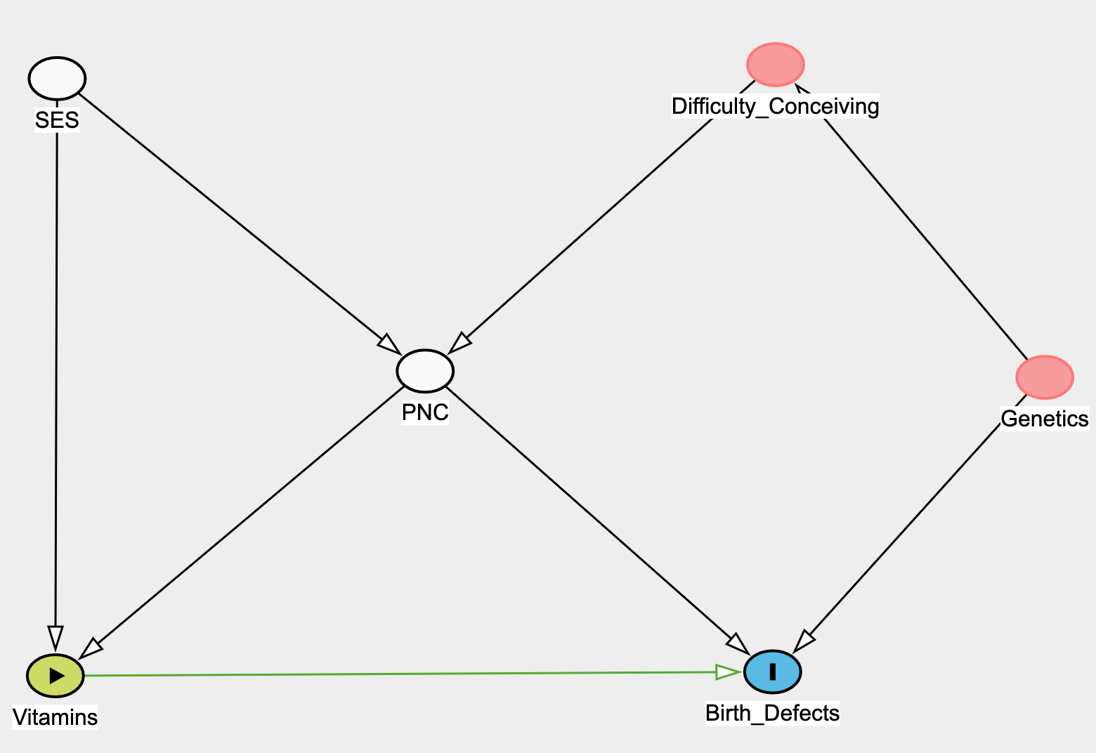
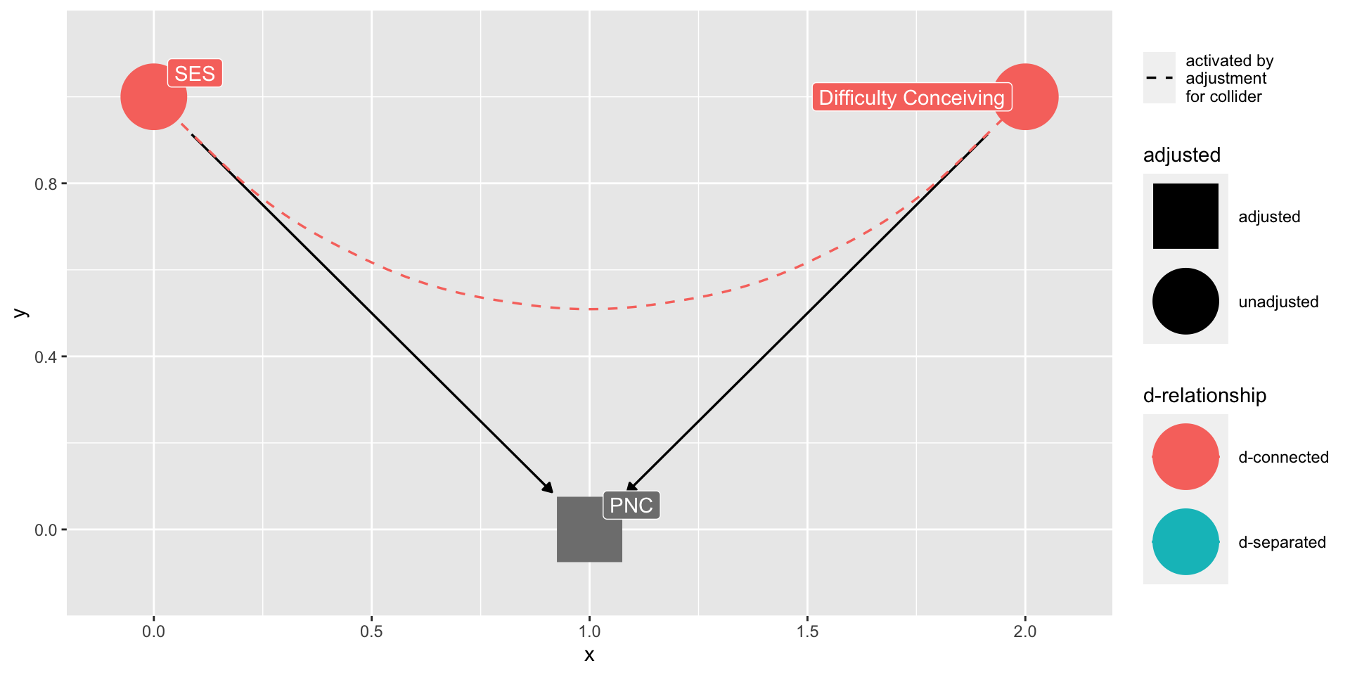
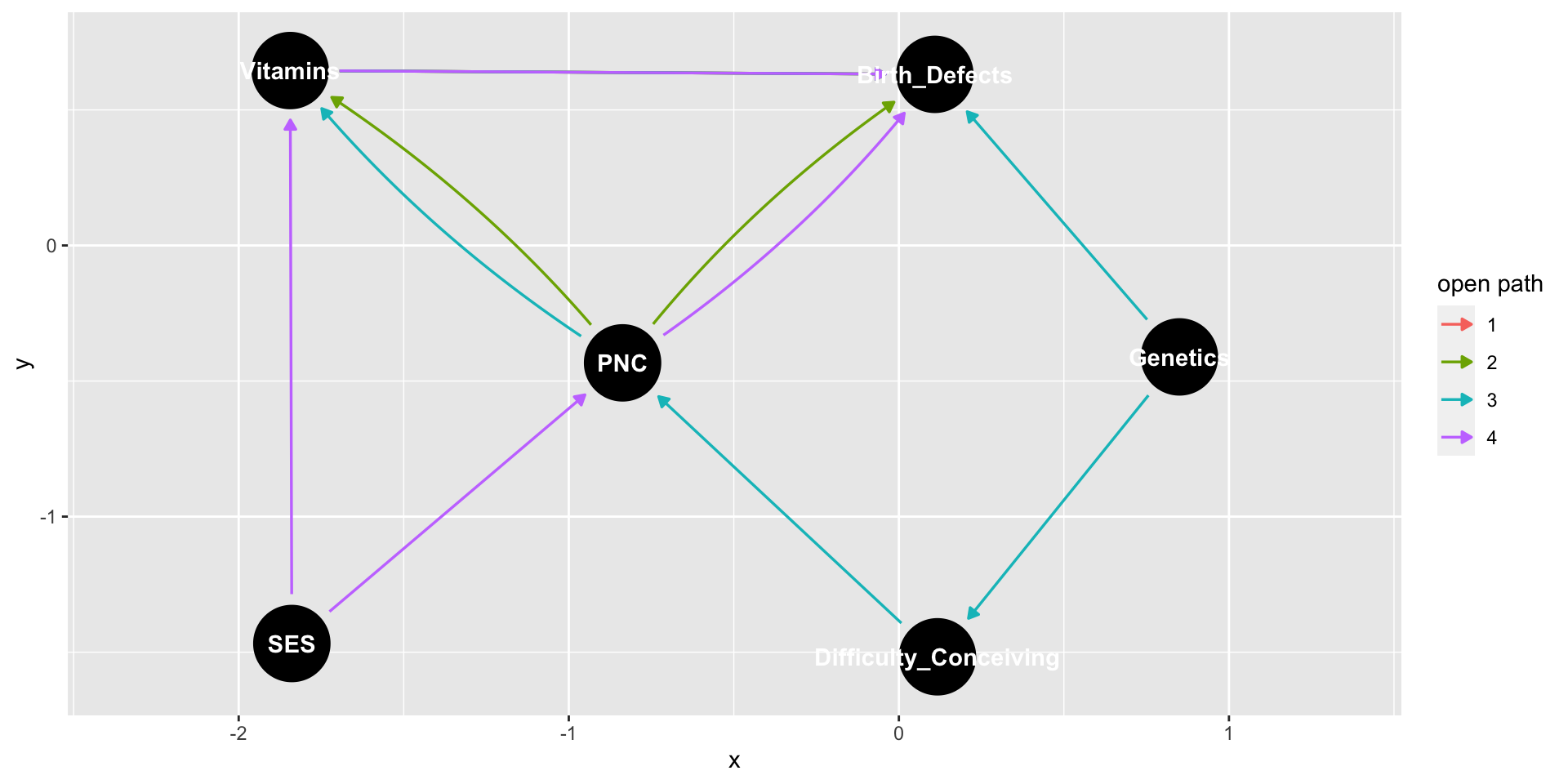
dag_cand3 %>% ggdag_paths(from = "Vitamins", to = "Birth_Defects",
                          adjust_for = "PNC", shadow = TRUE)

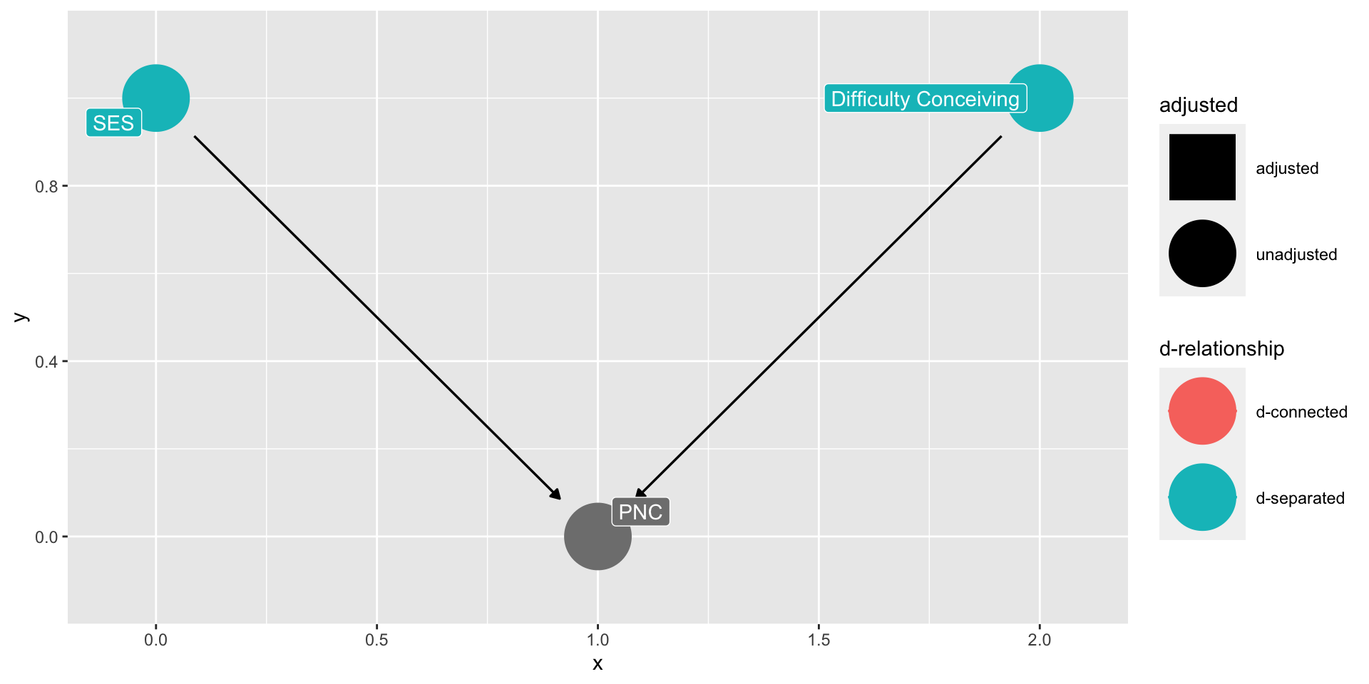
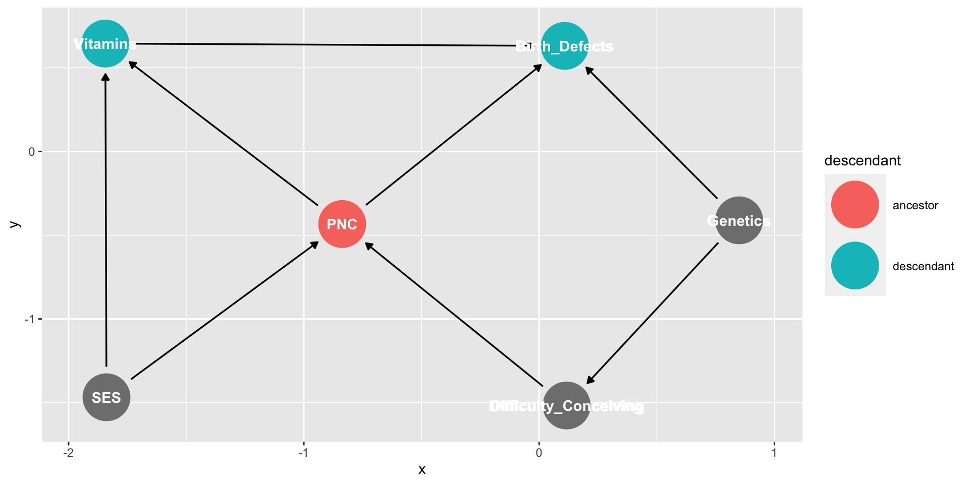
dag_cand3 %>% ggdag_dseparated(from = "Vitamins", to = "Birth_Defects", 
                               controlling_for = "PNC")

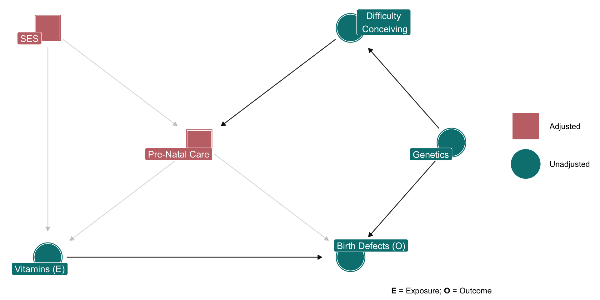
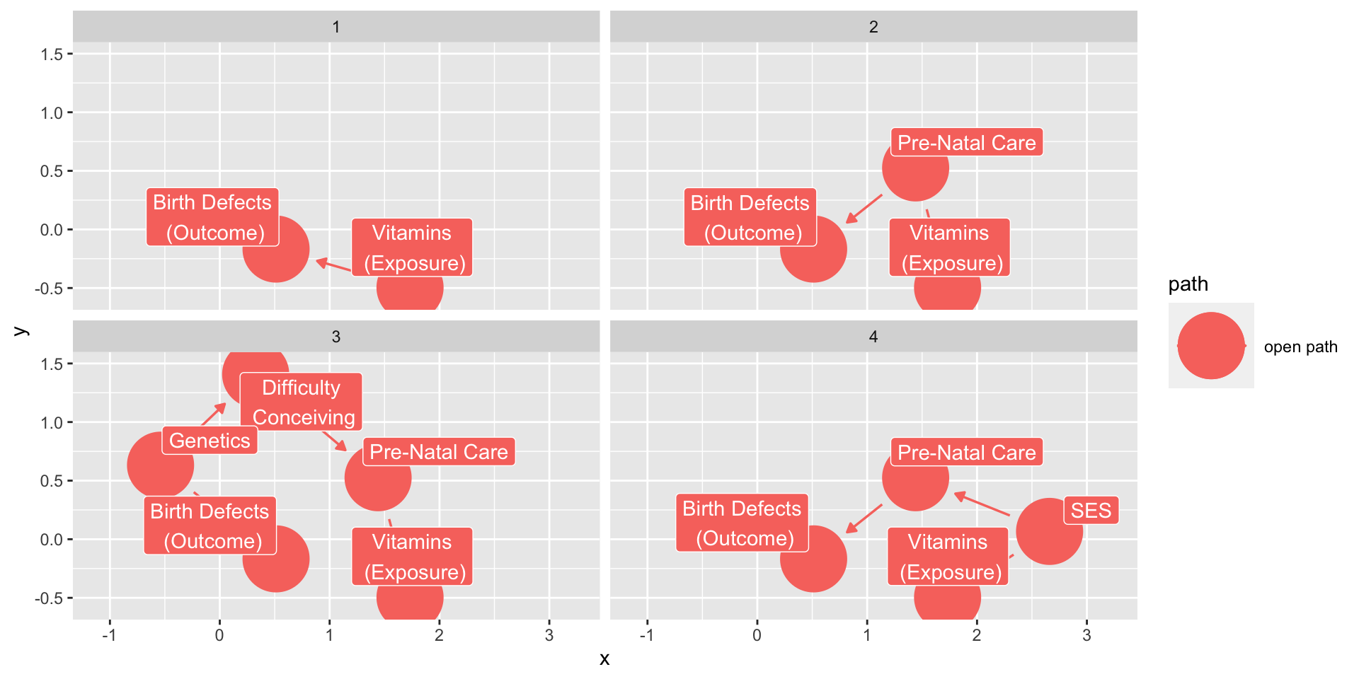
dag_cand3 %>% ggdag_paths(from = "Vitamins", to = "Birth_Defects",
                          adjust_for = c("PNC", "SES"), shadow = TRUE)

Customization via `ggdag` and `ggplot2`

Creating DAGs via `ggdag::dagify()`

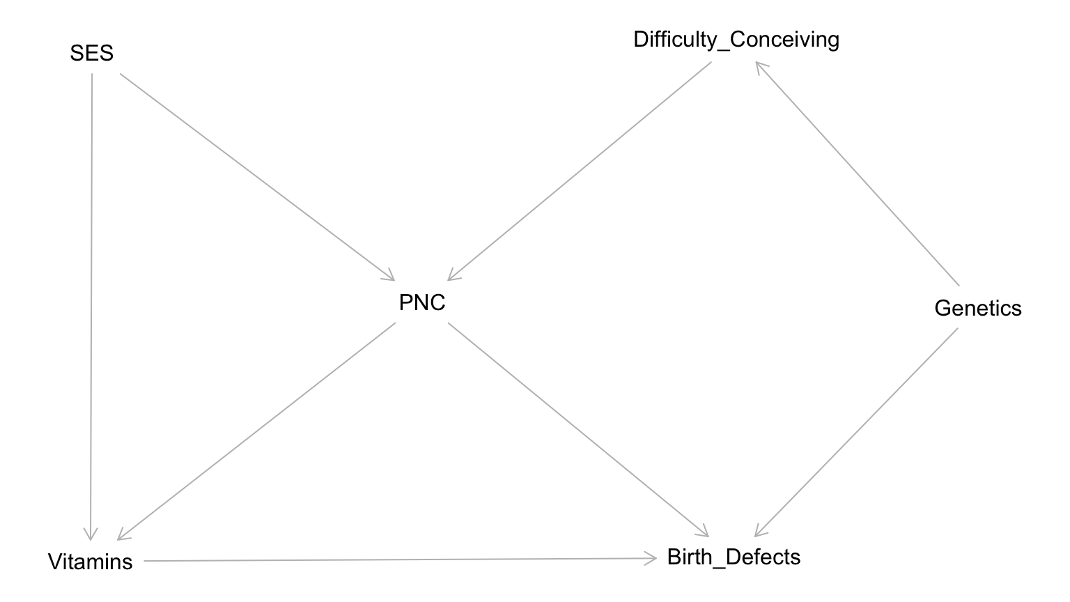
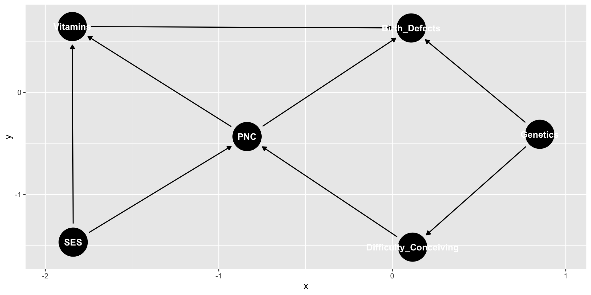
dag_cand3 <- dagify(#Here, we see conventional R syntax (e.g., outcome ~ predictors)
                    birth_defects ~ vitamins + pnc + genetics,
                    vitamins ~ ses + pnc,
                    pnc ~ ses + diff_conceiving,
                    diff_conceiving ~ genetics, 
                    exposure = "vitamins",
                    outcome = "birth_defects")

Creating DAGs via `ggdag::dagify()`

dag_cand3 <- dagify(#Here, we see conventional R syntax (e.g., outcome ~ predictors)
                    birth_defects ~ vitamins + pnc + genetics,
                    vitamins ~ ses + pnc,
                    pnc ~ ses + diff_conceiving,
                    diff_conceiving ~ genetics,
                    #These labels will be useful for plotting purposes down the line!
                    labels = c(#\n signals a line break
                               birth_defects = "Birth Defects\n (Outcome)",
                               vitamins = "Vitamins\n (Exposure)",
                               pnc = "Pre-Natal Care",
                               diff_conceiving = "Difficulty\n Conceiving",
                               ses = "SES",
                               genetics = "Genetics"),
                    exposure = "vitamins",
                    outcome = "birth_defects")

Using Labels

Base DAG
Identifying Open Paths
Identifying Covariate Adjustment Sets

set.seed(905)

dag_cand3 %>% ggdag(text = FALSE,
                    use_labels = "label")

set.seed(905)

dag_cand3 %>% ggdag_paths(text = FALSE,
                          use_labels = "label")

set.seed(905)

dag_cand3 %>% ggdag_adjustment_set(text = FALSE, 
                                   use_labels = "label") + 
              theme_dag()

Leveraging `ggplot2`

Step 1: Tidy DAG Object
Step 2: Use ggplot2 Functions

set.seed(905)

dag_cand3_gg <- dag_cand3 %>% 
                              tidy_dagitty(layout = "kk") %>% 
                              node_dconnected(controlling_for = c("pnc", "ses"))

dag_cand3_gg %>% slice(1:3)

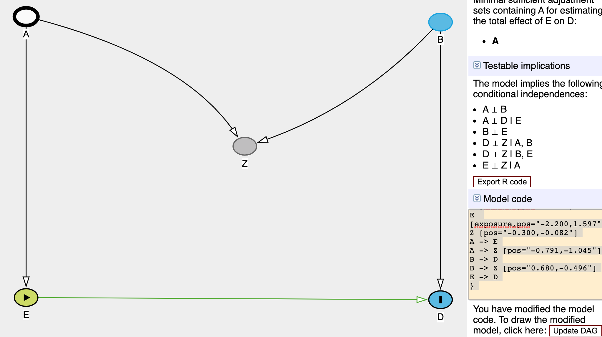
# A DAG with 3 nodes and 2 edges
#
# Exposure: vitamins
# Outcome: birth_defects
# Paths opened by conditioning on a collider: 
#
# A tibble: 3 × 12
  name        x     y direction to      xend   yend circular label collider_line
  <chr>   <dbl> <dbl> <fct>     <chr>  <dbl>  <dbl> <lgl>    <chr> <lgl>        
1 birth…  0.330 0.246 <NA>      <NA>  NA     NA     FALSE    "Bir… FALSE        
2 diff_… -0.891 0.399 ->        pnc   -0.373 -0.318 FALSE    "Dif… FALSE        
3 genet… -0.199 0.967 ->        birt…  0.330  0.246 FALSE    "Gen… FALSE        
# ℹ 2 more variables: adjusted <fct>, d_relationship <fct>

Show the underlying code

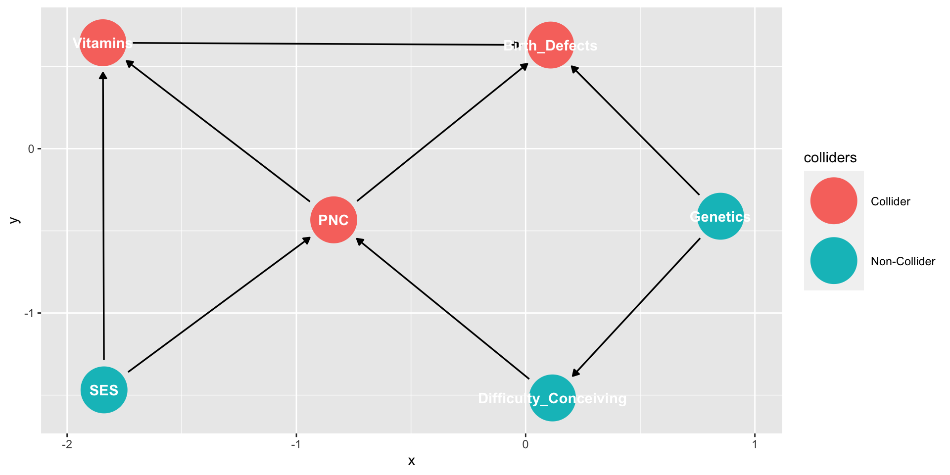
dag_cand3_gg %>% mutate(adjusted = #Simple way to capitalize a string:
                                    str_to_title(adjusted),
                        arrow = #Allows us to modify transparency of arrows as a function of whether or not a variable is adjusted:
                                    ifelse(adjusted == "Adjusted", 0.15, 0.85)) %>% 
                 ggplot(aes(#Coordinates (i.e., where the nodes will be located)
                             x = x, y = y, xend = xend, yend = yend, 
                             #Mapping aesthetics — will vary as a function of whether a variable is adjusted or unadjusted:
                             colour = adjusted, fill = adjusted, shape = adjusted)) +
                  #Adds nodes to plotting area:
                  ggdag::geom_dag_node() +
                  #Adds arrows connecting the nodes (as specified in your DAG syntax)::
                  geom_dag_edges(aes(#Adjusts transparency of arrows:
                                     edge_alpha = arrow), edge_width = 0.5) +
                  #Changes the shapes corresponding to adjusted/unadjusted.
                  scale_shape_manual(values = c(22, 21)) +
                  #The two lines that follow adjust the colour/fill of the nodes based on ggtheme's Economist theme:
                  scale_fill_economist() + scale_colour_economist() +
                  #The following line uses the logic of geom_label_repel to generate/modify your labels. 
                  geom_dag_label_repel(aes(label = label), colour = "white", show.legend = FALSE) +
                  theme_dag() +
                  #Removes legend title:
                  theme(legend.title = element_blank())

The End

sakeefkarim
sakeefkarim.com
code

A Quick Introduction to ggdag

What We’ll Do Today

A DAG Example

Pre-Natal Vitamins and Birth Defects

Using dagitty + ggdag

Step 1

Step 2

Step 3

Using ggdag as a Tool

Identifying Covariate Adjustment Sets

Identifying Colliders

Visualizing Collider Triangles

Visualizing Collider Triangles

Identifying A Variable’s Descendants

Identifying Open Paths

Identifying Open Paths

Customization via ggdag and ggplot2

Creating DAGs via ggdag::dagify()

Creating DAGs via ggdag::dagify()

Using Labels

Leveraging ggplot2

The End

A Quick Introduction to `ggdag`

Using `dagitty` + `ggdag`

Using `ggdag` as a Tool

Customization via `ggdag` and `ggplot2`

Creating DAGs via `ggdag::dagify()`

Creating DAGs via `ggdag::dagify()`

Leveraging `ggplot2`